Time to Code Part I

Aspects of Good Quality Code

Readable
Robust

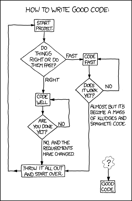
Source: xkcd

Code Readability: Whitespace

~~Code is for computers, comments are for humans.~~

While code must be syntactically correct for computers to execute, it should be formatted for humans to read and understand.

Use whitespace and newlines strategically to improve readability.

Compare:

Less Readable:

def calculate_risk(age,bp):risk=age*0.1+bp*0.05;return risk
patient_risk=calculate_risk(65,140);print(patient_risk)

More Readable:

def calculate_risk(age, bp):
    risk = age * 0.1 + bp * 0.05
    return risk

patient_age = 65
patient_bp = 140
patient_risk = calculate_risk(patient_age, patient_bp)
print(patient_risk)

Code Readability: Names

Use descriptive names for functions and variables.
- Start function names with a verb.
- Make variable names just long enough to be meaningful.

Compare:

Less Descriptive:

res <- mod(a, b)

More Descriptive:

risk_score <- calculate_risk(age, blood_pressure)

Code Readability: Consistency

Use a consistent coding style throughout your project.
- Consistency makes your code easier to understand and maintain.
- Consult a style guide for your programming language (keep conventions and avoid reinventing the wheel).

Compare:

Inconsistent Style:

def CalcRisk(Age,BP):
    risk_score=Age*0.1+BP*0.05
    Return risk_score

Consistent Style:

def calculate_risk(age, bp):
    risk_score = age * 0.1 + bp * 0.05
    return risk_score

Style Guides

Python Style Guide: PEP 8 – Style Guide for Python Code
R Style Guide: Tidyverse Style Guide

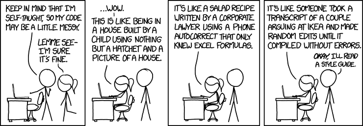
Source: xkcd

Linters

A linter is a static code analysis tool.

It scans your code and flags potential issues (style, errors, bugs).
It’s up to the programmer to review and fix the issues.

For Python:

flake8: Checks for style and programming errors.

For R:

lintr: Provides static code analysis for R.

Linters: Python

flake8 can be used to check your Python code for issues.

Usage:

flake8 path/to/your_code.py

Example:

Suppose you have the following code in calculate_risk.py:

def calculate_risk(age, bp):
    risk = age * 0.1 + bp * 0.05
    return risk

Running flake8 calculate_risk.py might output:

calculate_risk.py:2:1: E302 expected 2 blank lines, found 0
calculate_risk.py:2:6: E225 missing whitespace around operator
calculate_risk.py:3:1: E112 expected an indented block

These messages indicate where the code doesn’t conform to the style guide.

Linters: R

The lintr package can be used to check your R code.

Usage:

lintr::lint("path/to/your_code.R")

Example:

Suppose you have the following code in calculate_risk.R:

calculate_risk <- function(age,bp){
risk <- age*0.1 + bp*0.05
return(risk)
}

Running lintr::lint("calculate_risk.R") might output:

calculate_risk.R:1:31: style: Commas should always have a space after.
calculate_risk <- function(age,bp){
                                  ^
calculate_risk.R:2:9: style: Put spaces around all infix operators.
risk <- age*0.1 + bp*0.05
        ^

These messages help identify areas where the code can be improved for readability and consistency.

Autoformatters

While linters provide reports of issues, autoformatters automatically correct code formatting.

They modify your code directly to adhere to style guidelines.

For Python:

black: Formats code to follow PEP 8 style guidelines.

For R:

styler: Formats R code according to the Tidyverse style guide.

Autoformatters: Python

black can automatically format your Python code.

Usage:

black path/to/your_code.py

Example:

Given calculate_risk.py with inconsistent formatting:

def calculate_risk(age,bp):
  risk=age*0.1+bp*0.05
  return risk

Running black calculate_risk.py formats the code to:

def calculate_risk(age, bp):
    risk = age * 0.1 + bp * 0.05
    return risk

Autoformatters: R

The styler package can automatically format your R code.

Usage:

styler::style_file("path/to/your_code.R")

Example:

Given calculate_risk.R with inconsistent formatting:

calculate_risk <- function(age,bp){
  risk <- age*0.1+bp*0.05
  return(risk)
}

Running styler::style_file("calculate_risk.R") formats the code to:

calculate_risk <- function(age, bp) {
  risk <- age * 0.1 + bp * 0.05
  return(risk)
}

➡️ Exercise

Run a linter on your code to identify style issues:

Python: Use flake8 to analyze your code.

Install with pip install flake8.
Run flake8 your_code.py.

R: Use lintr to analyze your code.

Install with install.packages("lintr").
Run lintr::lint("your_code.R").

Edit your code to improve style compatibility based on the linter’s feedback.

Run an autoformatter to automatically fix style issues:

Python: Use black to format your code.

Install with pip install black.
Run black your_code.py.

R: Use styler to format your code.

Install with install.packages("styler").
Run styler::style_file("your_code.R").

Identify and note areas for improvement:

If you find code that is hard to read or variable names that need adjusting, make a note to work on it.
Use # TODO or another consistent label to mark areas for improvement.